
Training a neural network from scratch on limited data often produces disappointing results. The model struggles to learn meaningful patterns, overfits badly, or takes forever to train. You need thousands or millions of examples for deep learning to work well, but most real projects don’t have that luxury.
Leveraging pre-trained models through transfer learning lets you build powerful AI applications without massive datasets or computing resources. Instead of starting from random weights, you begin with a model that already learned useful features from millions of examples. This dramatically reduces training time and data requirements.
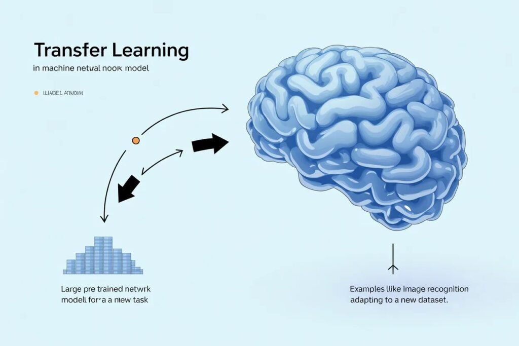
Transfer learning explained simply means taking knowledge learned from one task and applying it to a different but related task. A model trained on millions of images already knows how to detect edges, textures, shapes, and object parts. You adapt this knowledge to your specific problem rather than learning everything from scratch.
Why training from scratch often fails
Deep neural networks have millions or billions of parameters. Training these parameters to recognize patterns requires enormous amounts of data. ImageNet, the dataset used to train most computer vision models, contains 1.4 million images across 1,000 categories.
Most real projects have hundreds or thousands of examples, not millions. Training deep networks from scratch on small datasets leads to severe overfitting. The model memorizes training examples instead of learning generalizable patterns. It performs great on training data but fails on new examples.
Training from scratch also requires massive computational resources. ImageNet models train for days or weeks on multiple GPUs. Few individuals or small teams have access to this hardware. Even if you have the data and compute, training takes time you might not have.
The features learned in early layers of deep networks are surprisingly general. The first layers detect edges at different angles. Middle layers combine edges into textures and simple shapes. These low-level features apply across different visual tasks. You don’t need to relearn them for every project.
What makes transfer learning so powerful
Transfer learning works because different tasks share underlying structure. A model trained to classify ImageNet categories learned to see. It can detect objects, recognize textures, and understand spatial relationships. These skills transfer to classifying medical images, identifying plants, or detecting defects in manufacturing.
The pre-trained model acts as a feature extractor. Feed it an image and it produces rich numerical representations capturing what’s in that image. These representations already encode useful information learned from millions of training examples.
You add a small custom classifier on top of these features and train only that part on your specific data. Instead of learning millions of parameters from scratch, you learn a few thousand parameters for the classification head. This works with much less data because you’re only learning task-specific patterns, not general visual understanding.
Training is dramatically faster too. You freeze the pre-trained base and only update your custom head. This means far fewer parameters to optimize. What might take days training from scratch finishes in minutes or hours with transfer learning.
The quality of results improves substantially. Transfer learning models typically achieve 10 to 30 percent higher accuracy than training from scratch on the same small dataset. Sometimes the difference is even larger. This performance boost comes from leveraging knowledge encoded in the pre-trained weights.
Understanding feature extraction versus fine tuning

Transfer learning has two main approaches that work in different situations. Feature extraction freezes the entire pre-trained model and only trains the new classification head you add. Fine tuning unfreezes some or all of the pre-trained layers and trains them along with your custom head.
Feature extraction works when your task is similar to what the pre-trained model learned and you have limited data. The pre-trained features already capture what you need. You just learn to map those features to your specific classes.
from tensorflow import keras

# Load pre-trained model
base_model = keras.applications.MobileNetV2(
    input_shape=(224, 224, 3),
    include_top=False,
    weights='imagenet'
)

# Freeze all base model layers
base_model.trainable = False

# Add custom classification head
model = keras.Sequential([
    base_model,
    keras.layers.GlobalAveragePooling2D(),
    keras.layers.Dense(128, activation='relu'),
    keras.layers.Dropout(0.5),
    keras.layers.Dense(10, activation='softmax')
])

print(f"Trainable parameters: {sum([tf.size(w).numpy() for w in model.trainable_weights])}")
With feature extraction, only the classification head trains. The base model weights never change. This is fast and works well with small datasets because you’re learning far fewer parameters.
Fine tuning adapts the pre-trained features to your specific task. After initial training with frozen base, unfreeze some or all base layers and continue training with a very low learning rate. This gently adjusts features to work better for your data.
# After initial training with frozen base
base_model.trainable = True

# Freeze early layers, unfreeze later layers
for layer in base_model.layers[:100]:
    layer.trainable = False

# Compile with very low learning rate
model.compile(
    optimizer=keras.optimizers.Adam(1e-5),
    loss='categorical_crossentropy',
    metrics=['accuracy']
)

# Fine-tune
history = model.fit(train_data, epochs=5, validation_data=val_data)
Fine tuning works when you have more data and your task differs somewhat from the pre-trained model’s task. The low learning rate prevents destroying useful pre-trained weights. You’re making small adjustments rather than relearning from scratch.
Choosing the right pre-trained model
Many pre-trained models exist with different tradeoffs between accuracy, speed, and size. Choosing the right one depends on your constraints and requirements.
VGG models are older but simple and effective. They’re large and slow but achieve good accuracy. Use VGG if you have plenty of computational resources and prioritize accuracy over speed.
ResNet introduced residual connections that enable much deeper networks. ResNet50 and ResNet101 offer excellent accuracy and are widely used. They’re moderate size and speed. ResNet is a solid default choice for many applications.
MobileNet is optimized for mobile and embedded devices. It’s small and fast with acceptable accuracy. Use MobileNet when deploying to phones, edge devices, or when inference speed matters more than maximum accuracy.
EfficientNet achieves excellent accuracy with reasonable computational cost through carefully balanced scaling. It comes in multiple sizes from B0 (smallest) to B7 (largest). EfficientNet offers the best accuracy per computation and is great for production systems.
# Load different pre-trained models
vgg = keras.applications.VGG16(weights='imagenet', include_top=False)
resnet = keras.applications.ResNet50(weights='imagenet', include_top=False)
mobilenet = keras.applications.MobileNetV2(weights='imagenet', include_top=False)
efficientnet = keras.applications.EfficientNetB0(weights='imagenet', include_top=False)

# Compare parameter counts
models = [
    ('VGG16', vgg),
    ('ResNet50', resnet),
    ('MobileNetV2', mobilenet),
    ('EfficientNetB0', efficientnet)
]

for name, model in models:
    params = model.count_params()
    print(f"{name}: {params:,} parameters")
For NLP tasks, BERT and its variants are standard pre-trained models. They learned language understanding from massive text corpora. GPT models work well for text generation tasks. Use these instead of training language models from scratch.
When transfer learning works best
Transfer learning shines when you have limited labeled data for your specific task but abundant data exists for a related task. Computer vision benefits enormously because ImageNet provides a strong foundation for any visual task.
The source task and target task should be related. A model trained on natural images transfers well to medical images, satellite imagery, or product photos. The visual concepts overlap even though specific objects differ. A model trained on images doesn’t help with text classification because the domains are too different.
You need enough data to train the classification head even with transfer learning. A few dozen examples won’t work. Hundreds of examples per class is a reasonable minimum. Thousands per class gives good results. This is still far less than the millions needed to train from scratch.
Transfer learning works when your classes aren’t in the pre-trained model’s original training set. You can classify bird species even though ImageNet doesn’t have those exact species. The model learned bird-related features that transfer.
Practical tips for using transfer learning
Match input sizes to what the pre-trained model expects. Most ImageNet models expect 224 by 224 pixel images. Resize your images to match during preprocessing. Some models accept different sizes but matching the training size usually works best.
Apply the same preprocessing the pre-trained model was trained with. ImageNet models expect pixel values in specific ranges. Use the preprocessing function that comes with the model rather than writing your own.
from tensorflow.keras.applications.mobilenet_v2 import preprocess_input

# Correct preprocessing for MobileNetV2
img = keras.preprocessing.image.load_img('image.jpg', target_size=(224, 224))
img_array = keras.preprocessing.image.img_to_array(img)
img_array = preprocess_input(img_array)
Start with feature extraction before trying fine tuning. Train with the base frozen and see what accuracy you achieve. Only move to fine tuning if you need better performance and have sufficient data.
Use data augmentation to artificially increase your training set size. Rotate, flip, crop, and adjust brightness of images. This helps the model generalize better even with limited real examples.
Monitor both training and validation metrics during fine tuning. The low learning rate means training is slow. Stop if validation performance plateaus or degrades. You might be overfitting or the learning rate might be wrong.
Common mistakes to avoid
Don’t unfreeze all layers and train with a high learning rate. This destroys the pre-trained weights through drastic updates. Always use a very low learning rate for fine tuning, typically 10 to 100 times smaller than normal training.
Don’t forget to freeze the base model initially. If you train with all layers unfrozen from the start, you’re not doing transfer learning. You’re training from scratch with inconvenient initialization.
Don’t use transfer learning when you have massive amounts of data and compute. If you have millions of examples, training from scratch might work better. Transfer learning matters most when data is limited.
Don’t expect transfer learning to work across completely unrelated domains. A model trained on photographs won’t help with time series prediction. The domains must share some underlying structure for transfer to work.
Transfer learning explained through these concepts and techniques gives you a powerful tool for building AI applications without massive datasets. Pre-trained models encode knowledge from millions of examples. You adapt this knowledge to your specific task with minimal data and computation. This is how most production computer vision and NLP systems work today.
Ready to see transfer learning in action on a real project? Check out our cats vs dogs image classification tutorial where we build a classifier using transfer learning that achieves over 90 percent accuracy with a small dataset.