
You built your first neural network and it works reasonably well. But training takes forever, accuracy plateaus below where you want it, or the model overfits badly to training data. Basic architectures get you started, but professional-quality models require training techniques that address these common problems.
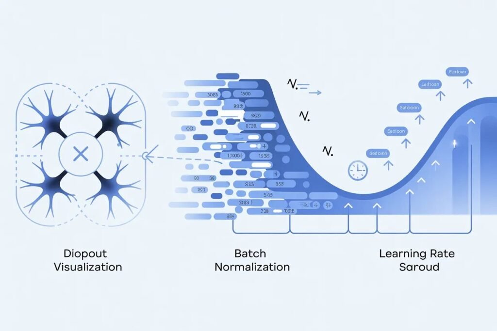
Mastering essential neural network training techniques transforms mediocre models into high-performing systems that train faster and generalize better. Three techniques stand out as must-know skills: dropout for preventing overfitting, batch normalization for faster convergence, and learning rate scheduling for optimal training progression.
Neural network training techniques like these separate amateur projects from production-quality models. They’re not complicated to implement with modern frameworks, but understanding when and how to use them makes a huge difference in your results. Let me show you exactly how each technique works and when to apply it.
Dropout prevents overfitting through randomness
Overfitting happens when your network memorizes training data instead of learning generalizable patterns. It performs great on training examples but poorly on new data. Dropout is one of the most effective techniques for preventing this.
Dropout works by randomly disabling neurons during training. For each training batch, dropout randomly sets some neuron outputs to zero with a specified probability. A dropout rate of 0.5 means each neuron has a 50 percent chance of being turned off during that batch.
This forces the network to learn robust features that work even when parts of the network are missing. No single neuron can become too important because it might be disabled at any moment. The network must distribute knowledge across many neurons.
Think of it like a sports team where random players sit out each game. The team must develop strategies that work regardless of which specific players are available. This creates a more resilient team overall.
During inference when making actual predictions, dropout is turned off. All neurons are active, but their outputs are scaled by the dropout rate to compensate for having more neurons active than during training.
from tensorflow import keras
from tensorflow.keras import layers
import numpy as np

# Model without dropout
model_basic = keras.Sequential([
    layers.Dense(128, activation='relu', input_shape=(784,)),
    layers.Dense(128, activation='relu'),
    layers.Dense(10, activation='softmax')
])

# Model with dropout
model_dropout = keras.Sequential([
    layers.Dense(128, activation='relu', input_shape=(784,)),
    layers.Dropout(0.5),  # Drop 50% of neurons
    layers.Dense(128, activation='relu'),
    layers.Dropout(0.5),
    layers.Dense(10, activation='softmax')
])

print("Basic model parameters:", model_basic.count_params())
print("Dropout model parameters:", model_dropout.count_params())
Add dropout layers after dense or convolutional layers where overfitting is a concern. Common dropout rates range from 0.2 to 0.5. Higher rates provide stronger regularization but might hurt model capacity if too aggressive.
Dropout works best when you have limited training data or complex models prone to overfitting. It’s less necessary with massive datasets where the model can’t easily memorize everything.
The technique is simple to implement but remarkably effective. Papers show dropout can reduce overfitting significantly and improve generalization, often matching or exceeding other regularization methods.
Batch normalization accelerates training
Training deep networks can be slow and unstable. Internal covariate shift is one reason. As weights update during training, the distribution of inputs to each layer keeps changing. This makes it hard for layers to learn effectively.
Batch normalization addresses this by normalizing layer inputs to have mean zero and standard deviation one. This happens for each mini-batch during training, keeping distributions stable throughout the network.
The technique adds a normalization step after the weighted sum but before the activation function. For each feature in the batch, subtract the batch mean and divide by the batch standard deviation. Then apply learnable scale and shift parameters.
This stabilization lets you use higher learning rates without training becoming unstable. Networks train faster because gradients flow more smoothly. It also acts as a regularizer, reducing the need for dropout in some cases.
# Model with batch normalization
model_batchnorm = keras.Sequential([
    layers.Dense(128, input_shape=(784,)),
    layers.BatchNormalization(),
    layers.Activation('relu'),

    layers.Dense(128),
    layers.BatchNormalization(),
    layers.Activation('relu'),

    layers.Dense(10, activation='softmax')
])

# Compile with higher learning rate
model_batchnorm.compile(
    optimizer=keras.optimizers.Adam(learning_rate=0.01),
    loss='categorical_crossentropy',
    metrics=['accuracy']
)

print("\nBatch normalization model summary:")
model_batchnorm.summary()
Place batch normalization layers after dense or convolutional layers but before activation functions. Some practitioners put it after activations, and both approaches can work. Experiment to see what works for your specific problem.
Batch normalization adds learnable parameters (scale and shift) for each feature. This slightly increases model size but the training speed improvement usually outweighs the cost.
The technique works particularly well for deep networks. Shallow networks with just a few layers might not benefit as much. For networks with 5 or more layers, batch normalization often provides noticeable improvements.
During inference, batch normalization uses running averages of mean and standard deviation computed during training rather than batch statistics. This ensures consistent predictions regardless of batch size.
Learning rate scheduling optimizes the training process
The learning rate controls how much weights change with each update. Too high and training becomes unstable. Too low and training crawls along slowly. The optimal learning rate often changes during training.
Learning rate scheduling adjusts the learning rate as training progresses. Common strategies include reducing the rate when improvement plateaus, exponentially decaying it over time, or following predefined schedules.
Starting with a higher learning rate makes rapid initial progress when the model is far from optimal. As training continues and the model approaches a good solution, reducing the learning rate helps fine-tune weights without overshooting.
Step decay reduces the learning rate by a factor every few epochs. You might multiply the learning rate by 0.1 every 30 epochs. This creates a staircase pattern where the rate drops at fixed intervals.
Exponential decay continuously reduces the learning rate by a small factor each epoch. The rate decreases smoothly rather than in discrete steps. The formula is: new rate equals initial rate times decay rate to the power of epoch number.
# Learning rate schedules
from tensorflow.keras.callbacks import LearningRateScheduler, ReduceLROnPlateau

# Step decay schedule
def step_decay_schedule(epoch, lr):
    if epoch > 0 and epoch % 10 == 0:
        return lr * 0.5
    return lr

# Exponential decay schedule
def exp_decay_schedule(epoch, lr):
    initial_lr = 0.001
    decay_rate = 0.95
    return initial_lr * (decay_rate ** epoch)

# Use schedule during training
lr_scheduler = LearningRateScheduler(step_decay_schedule)

model = keras.Sequential([
    layers.Dense(128, activation='relu', input_shape=(784,)),
    layers.Dense(10, activation='softmax')
])

model.compile(
    optimizer='adam',
    loss='categorical_crossentropy',
    metrics=['accuracy']
)

# Train with learning rate schedule
# history = model.fit(
#     X_train, y_train,
#     epochs=30,
#     callbacks=[lr_scheduler],
#     validation_split=0.2
# )
ReduceLROnPlateau is a practical callback that monitors validation metrics and reduces learning rate when improvement stalls. If validation loss doesn’t improve for a specified number of epochs, it reduces the learning rate automatically.
# Reduce learning rate when validation loss plateaus
reduce_lr = ReduceLROnPlateau(
    monitor='val_loss',
    factor=0.5,
    patience=5,
    min_lr=0.00001,
    verbose=1
)

# Use in training
# history = model.fit(
#     X_train, y_train,
#     epochs=50,
#     callbacks=[reduce_lr],
#     validation_split=0.2
# )
Cosine annealing is another popular schedule that follows a cosine curve. The learning rate decreases and increases cyclically, which can help escape local minima and find better solutions.
Choosing the right schedule depends on your problem and training dynamics. ReduceLROnPlateau is a safe default because it adapts automatically based on actual training progress.
Combining techniques for maximum impact
These techniques work even better together. Use dropout for regularization, batch normalization for training stability, and learning rate scheduling for optimal convergence.
A typical architecture might include batch normalization after each layer, dropout between dense layers, and a learning rate schedule that reduces the rate when validation performance plateaus.
# Complete model with all techniques
model_complete = keras.Sequential([
    layers.Dense(256, input_shape=(784,)),
    layers.BatchNormalization(),
    layers.Activation('relu'),
    layers.Dropout(0.3),

    layers.Dense(256),
    layers.BatchNormalization(),
    layers.Activation('relu'),
    layers.Dropout(0.3),

    layers.Dense(128),
    layers.BatchNormalization(),
    layers.Activation('relu'),
    layers.Dropout(0.3),

    layers.Dense(10, activation='softmax')
])

model_complete.compile(
    optimizer='adam',
    loss='categorical_crossentropy',
    metrics=['accuracy']
)

# Training with callbacks
callbacks = [
    ReduceLROnPlateau(
        monitor='val_loss',
        factor=0.5,
        patience=5,
        min_lr=0.00001
    ),
    keras.callbacks.EarlyStopping(
        monitor='val_loss',
        patience=10,
        restore_best_weights=True
    )
]

print("Complete model ready for training with all techniques")
Early stopping is another useful technique. It monitors validation performance and stops training when the model stops improving. This prevents wasting time on additional epochs that don’t help and reduces overfitting.
The combination of these techniques typically produces models that train faster, achieve higher accuracy, and generalize better than basic architectures. Expect 5 to 15 percent improvement in validation accuracy for many problems.
Practical guidelines for applying these techniques
Start with batch normalization if you’re training a deep network with more than 3 or 4 layers. It usually provides the biggest training speed improvement with minimal downside.
Add dropout if you see significant overfitting with training accuracy much higher than validation accuracy. Start with rates around 0.3 to 0.5 and adjust based on results.
Implement learning rate scheduling once basic training works. ReduceLROnPlateau is a good default that adapts automatically. More sophisticated schedules can help but require more tuning.
Don’t add all techniques at once without testing. Start with a baseline model, then add one technique at a time. Measure the impact of each addition so you know what actually helps.
Monitor both training and validation metrics. Techniques that improve training performance but hurt validation performance aren’t helping. The goal is better generalization, not just better training accuracy.
These neural network training techniques are standard practice in modern deep learning. They’re well supported by frameworks and backed by research showing real improvements. Learning to use them effectively makes you a more capable practitioner.
Ready to understand the decisions that go into building effective neural networks? Check out our guide on neural network optimization to learn how to choose the right optimizer, loss function, and activation function for your specific problem.