
You know that machine learning models learn from data and improve their predictions over time. But what’s actually happening during training? How does a model figure out which direction to adjust its parameters to get better results?
The answer is gradient descent, the optimization algorithm that powers almost every machine learning model you’ve ever used. Understanding how models optimize themselves through gradient descent is essential for grasping the learning process.
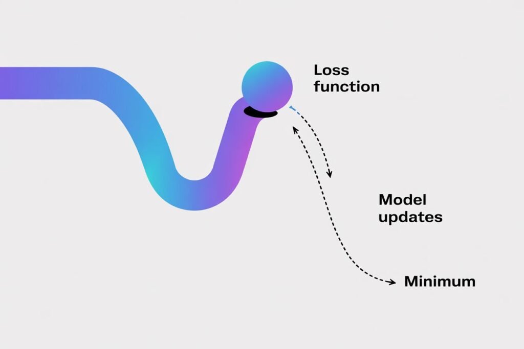
Gradient descent sounds complicated and mathematical, but the core concept is actually quite intuitive. Imagine you’re hiking down a mountain in thick fog. You can’t see the bottom, but you can feel which direction slopes downward. You take a step in that direction, feel the slope again, and keep walking downhill until you reach the valley.
That’s exactly what gradient descent does. The mountain is your loss function. The valley at the bottom represents the lowest possible loss. Your model takes small steps downhill until it finds the best parameters that minimize prediction errors.
The hill climbing analogy
Let me give you an even simpler way to think about gradient descent. Imagine you’re blindfolded at some random point on a hilly landscape. Your goal is to reach the lowest point you can find.
You can’t see where you are or where the lowest point is. But you can feel the slope of the ground beneath your feet. If the ground slopes down to your left, you know moving left will take you lower. If it slopes down to your right, you move right.
You take a small step in whichever direction slopes downward most steeply. Then you check the slope again from your new position. You keep taking steps downhill, one at a time, until you can’t find any direction that goes lower. You’ve reached a valley.
This is gradient descent. The height at any point represents your loss or error. The landscape shape is determined by your model’s parameters. Taking steps downhill means adjusting those parameters in whatever direction reduces the loss.
The gradient is just a fancy math term for the slope or direction of steepest descent. At any point, the gradient tells you which way is downhill and how steep it is. Your model calculates this gradient and moves in that direction.
A simple numerical example
Let’s walk through gradient descent with actual numbers so you can see exactly how it works. We’ll use the simplest possible example: finding the minimum of a basic function.
Suppose you have the function y equals x squared. This creates a U shaped curve. The lowest point is at x equals 0 where y equals 0. But pretend your model doesn’t know that. It starts at some random point and needs to find the minimum.
Let’s start at x equals 5. At this point, y equals 25. Our goal is to find the x value that gives us the lowest y value.
The slope of this function at any point is 2 times x. At x equals 5, the slope is 10. This positive slope means the function is going upward to the right. To go downhill, we need to move left, which means decreasing x.
We set a learning rate of 0.1. This controls how big our steps are. Our update rule is: new x equals old x minus learning rate times slope.
Step 1: x equals 5, slope equals 10. New x equals 5 minus 0.1 times 10 equals 4. We moved from 5 to 4.
Step 2: x equals 4, slope equals 8. New x equals 4 minus 0.1 times 8 equals 3.2. We moved from 4 to 3.2.
Step 3: x equals 3.2, slope equals 6.4. New x equals 3.2 minus 0.1 times 6.4 equals 2.56.
Notice we’re getting closer to x equals 0 with each step. The steps also get smaller as we approach the minimum because the slope gets less steep.
If we continue this process, x converges toward 0, which is indeed the minimum of the function. This is gradient descent in action.
import numpy as np

def function(x):
    return x ** 2

def gradient(x):
    return 2 * x

# Starting point
x = 5.0
learning_rate = 0.1

# Perform gradient descent
for step in range(20):
    grad = gradient(x)
    x = x - learning_rate * grad
    print(f"Step {step + 1}: x = {x:.4f}, f(x) = {function(x):.4f}")
This code shows gradient descent finding the minimum of x squared. Run it and watch how x approaches zero and the function value approaches its minimum.
How learning rate affects the process
The learning rate is one of the most important settings in gradient descent. It controls how big each step is as your model moves toward the minimum.
If your learning rate is too small, your model takes tiny steps. It will eventually reach the minimum but it takes forever. You might need millions of iterations to get there. This is inefficient and wastes time and computing resources.
If your learning rate is too large, your model takes huge steps. It might overshoot the minimum completely. Imagine trying to walk down a narrow valley by taking giant leaps. You’d jump from one side to the other, never settling at the bottom.
With an overly large learning rate, your loss might actually increase instead of decrease. The model jumps past the minimum to somewhere higher up on the other side. It can even diverge completely, with loss growing larger and larger.
Finding the right learning rate requires experimentation. Common values range from 0.001 to 0.1, but the optimal value depends on your specific problem. Many machine learning frameworks use adaptive learning rates that automatically adjust during training.
# Comparing different learning rates
learning_rates = [0.01, 0.1, 0.5, 1.1]

for lr in learning_rates:
    x = 5.0
    print(f"\nLearning rate: {lr}")

    for step in range(5):
        grad = gradient(x)
        x = x - lr * grad
        print(f"  Step {step + 1}: x = {x:.4f}")
This code demonstrates how different learning rates affect convergence. The 0.01 rate is too slow. The 1.1 rate overshoots and diverges. The 0.1 rate works well.
Gradient descent in real machine learning
In actual machine learning models, gradient descent works the same way but with many more parameters. Instead of finding the minimum of a simple function with one variable, you’re optimizing hundreds or millions of parameters simultaneously.
A neural network might have millions of weights and biases. Gradient descent adjusts all of them together, calculating how each parameter should change to reduce the overall loss.
The gradient becomes a vector pointing in the direction of steepest increase in your high dimensional parameter space. You move in the opposite direction of that vector to go downhill.
The process works identically to our simple example. Calculate the current loss. Compute the gradient with respect to all parameters. Update each parameter by moving a small step in the direction that reduces loss. Repeat thousands of times until the loss stops decreasing.
Modern deep learning uses variations of basic gradient descent. Stochastic gradient descent updates parameters using small batches of data instead of the entire dataset at once. This speeds up training significantly.
Momentum based methods remember previous gradients and build up velocity in consistent directions. This helps the model move faster through flat regions and escape shallow local minima.
Adam and other adaptive methods automatically adjust the learning rate for each parameter based on recent gradients. These optimizers often work better than plain gradient descent with less tuning required.
from sklearn.linear_model import SGDRegressor
import numpy as np

# Sample data
X = np.array([[1], [2], [3], [4], [5]])
y = np.array([2, 4, 6, 8, 10])

# Model using stochastic gradient descent
model = SGDRegressor(learning_rate='constant', eta0=0.01, max_iter=1000)
model.fit(X, y)

print(f"Learned coefficient: {model.coef_[0]:.4f}")
print(f"Learned intercept: {model.intercept_[0]:.4f}")
This example shows sklearn using gradient descent to learn a simple linear relationship. The model finds parameters that best fit the data through iterative optimization.
Common problems and solutions
Gradient descent doesn’t always work perfectly. Several issues can prevent it from finding good solutions.
Local minima are valleys that aren’t the deepest point overall. Your model can get stuck in a local minimum and never find the global minimum. This is less of a problem with neural networks than you might expect because high dimensional spaces have fewer true local minima than intuition suggests.
Saddle points look like minima in some directions but maxima in others. Gradient descent can slow down dramatically near saddle points because the gradient becomes very small. Momentum helps push through these flat regions.
Vanishing gradients occur in deep neural networks when gradients become extremely small in early layers. Updates become so tiny that learning essentially stops. Modern architectures and techniques like batch normalization help address this.
Exploding gradients are the opposite problem where gradients become huge, causing wild parameter updates. Gradient clipping limits gradient magnitude to prevent this instability.
Choosing good initial parameter values helps gradient descent start from a reasonable location. Random initialization works well with proper scaling. Starting too far from good solutions can make convergence slow or impossible.
Why gradient descent matters
Understanding gradient descent explained simply gives you insight into the core mechanism behind machine learning. Every time you train a model, gradient descent is working behind the scenes to minimize loss and improve predictions.
The algorithm’s simplicity is beautiful. By repeatedly taking small steps downhill, models with millions of parameters can learn complex patterns from data. You don’t need to manually figure out the right parameter values. Gradient descent finds them automatically through optimization.
This optimization process is what lets machine learning models improve from experience. The model makes predictions, measures how wrong they are, and adjusts itself to be less wrong next time. Repeat this process enough times and you get a model that works.
Different machine learning algorithms use variations of gradient descent, but the fundamental idea remains the same. Follow the gradient downhill to minimize your objective function. This core concept powers everything from simple linear regression to massive neural networks.
Now that you understand how models optimize themselves through gradient descent, you’re ready to put these concepts together. Want to see all these pieces working in practice? Check out our guide on how to build your first machine learning model in Python to create a complete working system from scratch.