
You know that neural networks learn from data and make predictions. But what actually happens when you feed an input into a trained network? How does it transform your data through layers of neurons to produce an output?
Understanding how neural networks process information through forward propagation is essential for anyone learning deep learning. This is the mechanism that takes your input data and produces predictions. It’s the forward journey through the network that happens every time you use a trained model.
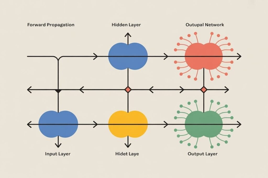
Forward propagation explained simply is the process of passing input data through each layer of a neural network, applying mathematical operations at each step, until reaching the final output. Data flows in one direction from input to output, hence the name forward propagation. Let me show you exactly what happens at each step.
The journey from input to output
Imagine you have a simple neural network with 3 input neurons, 2 hidden neurons, and 1 output neuron. You want to predict whether a customer will buy a product based on three features: age, income, and time spent on website.
Your input is a vector of three numbers representing these features. Maybe age equals 35, income equals 50000, and time equals 10 minutes. These three values enter the input layer.
The input layer doesn’t do any computation. It just holds your data and passes it forward to the first hidden layer. Think of it as a staging area that receives your data in the format the network expects.
From the input layer, data flows to the hidden layer. Each hidden neuron receives all three input values. This is where the first real computation happens.
Each hidden neuron has weights connecting it to each input. Hidden neuron 1 might have weights of 0.5, 0.3, and 0.8 for age, income, and time respectively. These weights were learned during training and determine how much each input influences this neuron.
The neuron calculates a weighted sum. Multiply each input by its corresponding weight and add them together. For our example: 35 times 0.5 plus 50000 times 0.3 plus 10 times 0.8 equals 15008.5.
Then add the bias term. Every neuron has a bias that shifts its activation threshold. If the bias is 1.2, the weighted sum becomes 15009.7.
Finally, apply the activation function. If using ReLU, the output is max(0, 15009.7) which equals 15009.7. If the weighted sum had been negative, ReLU would output 0.
This entire process repeats for each neuron in the hidden layer. Hidden neuron 2 has different weights, calculates its own weighted sum, adds its own bias, and applies the activation function.
import numpy as np

def forward_propagation_step_by_step():
    # Input data
    age = 35
    income = 50000
    time = 10
    inputs = np.array([age, income, time])

    # Hidden neuron 1 weights and bias
    weights_h1 = np.array([0.5, 0.3, 0.8])
    bias_h1 = 1.2

    # Calculate weighted sum
    weighted_sum_h1 = np.dot(inputs, weights_h1) + bias_h1
    print(f"Hidden neuron 1 weighted sum: {weighted_sum_h1:.2f}")

    # Apply ReLU activation
    activation_h1 = max(0, weighted_sum_h1)
    print(f"Hidden neuron 1 activation: {activation_h1:.2f}")

    # Hidden neuron 2 weights and bias
    weights_h2 = np.array([0.2, 0.1, 0.6])
    bias_h2 = 0.5

    weighted_sum_h2 = np.dot(inputs, weights_h2) + bias_h2
    activation_h2 = max(0, weighted_sum_h2)
    print(f"Hidden neuron 2 activation: {activation_h2:.2f}")

    return activation_h1, activation_h2

h1_out, h2_out = forward_propagation_step_by_step()
Now you have outputs from the hidden layer. These become inputs to the output layer. The output neuron receives the two hidden layer outputs and repeats the same process: weighted sum, add bias, apply activation.
For binary classification, the output layer typically uses sigmoid activation to produce a probability between 0 and 1. An output of 0.8 means the network predicts an 80 percent chance the customer will buy.
Matrix mathematics make it efficient
Walking through individual neurons helps understand the concept, but neural networks use matrix operations to compute everything simultaneously. This is much faster, especially with GPUs designed for matrix calculations.
Instead of processing one neuron at a time, you organize weights into a matrix. Each row represents one neuron’s weights. Multiply the input vector by this weight matrix in one operation to get all weighted sums at once.
For our example, the hidden layer weight matrix has 2 rows (one per hidden neuron) and 3 columns (one per input). Matrix multiplication of inputs times weights gives you both weighted sums simultaneously.
def forward_propagation_with_matrices():
    # Input data
    inputs = np.array([35, 50000, 10])

    # Weight matrix for hidden layer (2 neurons, 3 inputs each)
    W_hidden = np.array([
        [0.5, 0.3, 0.8],  # neuron 1 weights
        [0.2, 0.1, 0.6]   # neuron 2 weights
    ])

    # Bias vector for hidden layer
    b_hidden = np.array([1.2, 0.5])

    # Calculate weighted sums for all hidden neurons at once
    z_hidden = np.dot(W_hidden, inputs) + b_hidden
    print(f"Hidden layer weighted sums: {z_hidden}")

    # Apply ReLU activation to all at once
    a_hidden = np.maximum(0, z_hidden)
    print(f"Hidden layer activations: {a_hidden}")

    # Output layer weights and bias
    W_output = np.array([0.4, 0.7])
    b_output = 0.3

    # Output layer calculation
    z_output = np.dot(W_output, a_hidden) + b_output

    # Sigmoid activation for binary classification
    a_output = 1 / (1 + np.exp(-z_output))
    print(f"Final output (probability): {a_output:.4f}")

    return a_output

prediction = forward_propagation_with_matrices()
This matrix approach computes the same results but much faster. Modern deep learning frameworks like TensorFlow and PyTorch use highly optimized matrix operations that run on GPUs, processing thousands of examples in parallel.
Layer by layer through a deep network
Real neural networks often have many hidden layers. Forward propagation simply repeats the same process for each layer. The output of one layer becomes the input to the next layer.
A deep network with 5 hidden layers processes data through 7 total layers: input, 5 hidden, and output. At each hidden layer, you compute weighted sums, add biases, and apply activations. Each layer transforms the data representation.
Early layers might learn simple patterns. In image recognition, the first layer might detect edges. The second layer combines edges into shapes. The third layer combines shapes into object parts. Later layers recognize complete objects.
This hierarchical feature learning is why deep networks work so well. Each layer builds on representations from previous layers, creating increasingly abstract and powerful features.
The computation flows smoothly from input to output without any loops or backward steps. That’s why it’s called forward propagation. Information moves forward through the network in a single pass.
Why forward propagation matters
Forward propagation is how trained neural networks make predictions on new data. When you deploy a model to production, forward propagation is what runs billions of times to serve predictions.
Understanding forward propagation helps you debug networks. If your network produces strange outputs, you can trace the forward pass to see where values become unusual. Maybe one layer outputs extremely large values due to initialization or missing normalization.
It also helps you understand computational costs. The number of parameters (weights and biases) and the number of operations per layer determine how fast forward propagation runs. Larger networks with more layers take longer.
Batch processing leverages matrix operations to process multiple examples simultaneously. Instead of one input vector, you have a matrix where each row is one example. The same forward propagation calculations work on the entire batch at once, maximizing GPU utilization.
def forward_prop_batch():
    # Batch of 4 examples
    batch_inputs = np.array([
        [35, 50000, 10],
        [25, 30000, 5],
        [45, 80000, 15],
        [55, 60000, 8]
    ])

    # Same weights as before
    W_hidden = np.array([
        [0.5, 0.3, 0.8],
        [0.2, 0.1, 0.6]
    ])
    b_hidden = np.array([1.2, 0.5])

    # Process entire batch at once
    z_hidden = np.dot(batch_inputs, W_hidden.T) + b_hidden
    a_hidden = np.maximum(0, z_hidden)

    print(f"Batch hidden activations shape: {a_hidden.shape}")
    print(f"First example hidden activations: {a_hidden[0]}")

    return a_hidden

batch_results = forward_prop_batch()
Batch processing is standard in training and inference. It’s much more efficient than processing examples one at a time.
Common mistakes and how to avoid them
Shape mismatches cause frequent errors in forward propagation. Your weight matrix dimensions must align with input dimensions. If you have 10 inputs, each hidden neuron needs 10 weights. The weight matrix for 5 hidden neurons must be 5 by 10.
Forgetting to apply activation functions breaks the network’s ability to learn non-linear patterns. Without activations, your deep network reduces to a single linear transformation. Always apply activations after weighted sums.
Using the wrong activation function for the output layer produces nonsensical predictions. Binary classification needs sigmoid or softmax. Regression needs no activation or ReLU. Multi-class classification needs softmax.
Not normalizing inputs causes training problems. If one input ranges from 0 to 1 and another from 0 to 1000000, the large values dominate gradients. Normalize or standardize inputs before feeding them to the network.
Numerical instability can occur with certain activations or very large networks. The sigmoid activation can output values so close to 0 or 1 that they cause numerical issues. Modern activations like ReLU avoid most of these problems.
Forward propagation in practice
When using deep learning frameworks, you rarely implement forward propagation manually. The framework handles it automatically when you call model.predict() or during training.
But understanding what happens under the hood helps you design better architectures, debug problems, and optimize performance. You know that adding layers increases computation. You understand why batch size affects memory usage.
Forward propagation explained shows you the exact mathematical journey data takes through your network. From input values to weighted sums to activations to final outputs, each step transforms the data representation.
This forward pass happens during both training and inference. During training, forward propagation produces predictions that are compared to true labels. The error drives the backward pass that updates weights. But that’s a topic for backpropagation.
Ready to understand how neural networks actually learn and improve? Check out our guide on backpropagation for beginners to see how networks calculate gradients and update weights to minimize prediction errors through the learning process.