Forward propagation shows you how neural networks make predictions. But how do they get better at those predictions? How does a network that starts with random weights learn to recognize images, understand language, or predict outcomes accurately?
Learning how neural networks improve through backpropagation reveals the training process that makes deep learning possible. This is the algorithm that adjusts weights based on errors, gradually transforming a random network into one that makes useful predictions. Understanding backpropagation helps you train better models and debug training problems.
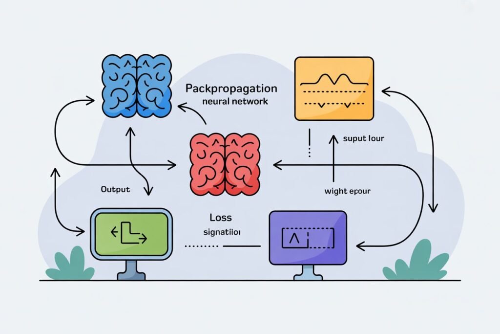
Backpropagation for beginners means understanding how neural networks calculate gradients and update weights to reduce errors. The network makes predictions, measures how wrong they are, then works backward through layers to figure out how to adjust each weight. Let me break down this learning process step by step.
The learning cycle that makes networks smarter
Neural networks learn through repeated cycles. Make a prediction with forward propagation. Compare the prediction to the true answer. Calculate how wrong you were. Use that error to update weights. Repeat thousands or millions of times until the network makes good predictions.
Backpropagation handles the crucial step of figuring out how to update weights. After forward propagation produces a prediction, you calculate the loss or error. If predicting whether a customer will buy and the network outputs 0.8 but the customer didn’t buy, the error is significant.
The loss function quantifies this error mathematically. For binary classification, binary cross entropy measures how far predicted probabilities are from true labels. For regression, mean squared error measures the squared difference between predictions and actual values.
Once you know the total error, backpropagation answers a critical question: how should each weight change to reduce that error? Which weights contributed most to the mistake? How much should each weight increase or decrease?
This requires calculating the gradient of the loss with respect to every weight in the network. The gradient tells you the direction and magnitude that each weight should change to reduce loss.
The chain rule makes backpropagation work
Backpropagation uses the chain rule from calculus to calculate gradients efficiently. Don’t worry if you’re not comfortable with calculus. The intuition is more important than the detailed math.
The chain rule says that if you have a chain of operations, you can find how the final output changes with respect to early inputs by multiplying derivatives along the chain.
Think about a simple example. You have x, you calculate y equals 2 times x, then you calculate z equals y squared. How does z change when x changes? The chain rule says multiply the derivatives: dz/dx equals dz/dy times dy/dx.
Neural networks are chains of operations. Input goes through weighted sum, then activation, then another weighted sum, then another activation, continuing through all layers until the final output and loss calculation.
To find how loss changes with respect to a weight in the first layer, you multiply derivatives backward through all these operations. Start with how loss changes with respect to the final output. Multiply by how that output changes with respect to the previous layer. Continue backward until you reach the weight you care about.
This backward calculation is why it’s called backpropagation. You propagate error gradients backward through the network from output to input.
import numpy as np

# Simple backprop example with one layer
def simple_backprop_example():
    # Forward pass
    x = np.array([1.0, 2.0])  # inputs
    w = np.array([0.5, 0.3])  # weights
    b = 0.1  # bias

    # Weighted sum
    z = np.dot(x, w) + b
    print(f"Weighted sum: {z:.4f}")

    # Sigmoid activation
    a = 1 / (1 + np.exp(-z))
    print(f"Activation (prediction): {a:.4f}")

    # True label
    y_true = 1

    # Loss (binary cross entropy simplified)
    loss = -(y_true * np.log(a) + (1 - y_true) * np.log(1 - a))
    print(f"Loss: {loss:.4f}")

    # Backward pass
    # Gradient of loss with respect to activation
    dL_da = -(y_true / a) + (1 - y_true) / (1 - a)

    # Gradient of activation with respect to weighted sum
    da_dz = a * (1 - a)

    # Gradient of loss with respect to weighted sum
    dL_dz = dL_da * da_dz

    # Gradient of loss with respect to weights
    dL_dw = dL_dz * x

    # Gradient of loss with respect to bias
    dL_db = dL_dz

    print(f"\nGradients:")
    print(f"dL/dw: {dL_dw}")
    print(f"dL/db: {dL_db:.4f}")

    return dL_dw, dL_db

gradients_w, gradient_b = simple_backprop_example()
This code shows backpropagation for one neuron. The forward pass calculates the prediction and loss. The backward pass calculates gradients by applying the chain rule step by step.
Updating weights with gradient descent
Once you have gradients for all weights, you update them using gradient descent. The gradient tells you which direction increases loss. You move in the opposite direction to decrease loss.
The update rule is simple: new weight equals old weight minus learning rate times gradient. The learning rate controls how big each step is. Too large and training becomes unstable. Too small and training takes forever.
If a weight has a gradient of 0.5 and your learning rate is 0.01, you subtract 0.01 times 0.5 equals 0.005 from the weight. The weight decreases slightly, which should reduce loss on the next forward pass.
Positive gradients mean increasing the weight increases loss, so you decrease the weight. Negative gradients mean increasing the weight decreases loss, so you increase the weight.
def gradient_descent_update():
    # Initial weights from previous example
    w = np.array([0.5, 0.3])
    b = 0.1

    # Gradients from backprop
    dL_dw = np.array([0.2, 0.4])  # example gradients
    dL_db = 0.3

    # Learning rate
    learning_rate = 0.01

    # Update weights
    w_new = w - learning_rate * dL_dw
    b_new = b - learning_rate * dL_db

    print(f"Original weights: {w}")
    print(f"Updated weights: {w_new}")
    print(f"Original bias: {b:.4f}")
    print(f"Updated bias: {b_new:.4f}")

    return w_new, b_new

updated_w, updated_b = gradient_descent_update()
This update happens for every weight and bias in the network after each batch of training examples. Over thousands of updates, weights gradually adjust to reduce loss and improve predictions.
The complete training loop
Training a neural network combines forward propagation, loss calculation, backpropagation, and weight updates into a repeated cycle.
First, initialize all weights randomly. Random initialization breaks symmetry so different neurons learn different features. Common approaches use small random values from a normal or uniform distribution.
Then loop through your training data many times. Each complete pass through all training data is called an epoch. You typically train for tens or hundreds of epochs.
For each batch of training examples, run forward propagation to get predictions. Calculate loss comparing predictions to true labels. Run backpropagation to calculate gradients. Update all weights using gradient descent.
Track the loss as training progresses. Loss should generally decrease over time. If it’s not decreasing, your learning rate might be wrong, your network architecture might be inappropriate, or your data might have issues.
# Simplified training loop structure
def training_loop_example(X_train, y_train, epochs=10, batch_size=32, learning_rate=0.01):
    # Initialize weights randomly
    # (actual implementation would depend on network architecture)

    n_samples = len(X_train)

    for epoch in range(epochs):
        epoch_loss = 0

        # Process data in batches
        for i in range(0, n_samples, batch_size):
            batch_X = X_train[i:i+batch_size]
            batch_y = y_train[i:i+batch_size]

            # Forward propagation
            predictions = forward_pass(batch_X)

            # Calculate loss
            loss = calculate_loss(predictions, batch_y)
            epoch_loss += loss

            # Backpropagation
            gradients = backward_pass(loss)

            # Update weights
            update_weights(gradients, learning_rate)

        avg_loss = epoch_loss / (n_samples / batch_size)
        print(f"Epoch {epoch+1}/{epochs}, Loss: {avg_loss:.4f}")

# Note: forward_pass, calculate_loss, backward_pass, update_weights
# are placeholder functions representing the actual operations
This structure forms the backbone of neural network training. Frameworks like TensorFlow and PyTorch implement these steps efficiently, handling the complex mathematics automatically.
Common training problems and solutions
Vanishing gradients occur when gradients become extremely small in early layers of deep networks. Each layer multiplies gradients during backpropagation. With many layers and certain activation functions, gradients can become so small that early layers barely update.
ReLU activations help prevent vanishing gradients. Unlike sigmoid which has gradients near zero for large positive or negative inputs, ReLU has a gradient of 1 for positive inputs. This keeps gradients from shrinking too much.
Exploding gradients are the opposite problem where gradients become extremely large, causing huge weight updates that destabilize training. Gradient clipping limits gradient magnitude to prevent this. If gradients exceed a threshold, scale them down.
Choosing the right learning rate is critical. Too high causes oscillation or divergence. Too low makes training painfully slow. Learning rate schedules that decrease the learning rate over time often work well. Start with a larger rate for fast initial progress, then decrease for fine tuning.
Overfitting happens when the network memorizes training data instead of learning generalizable patterns. Regularization techniques like dropout and L2 penalties on weights help prevent overfitting by discouraging the network from relying too heavily on any single weight.
Why backpropagation matters
Backpropagation is the algorithm that made modern deep learning possible. Before backpropagation, training neural networks was inefficient and limited to shallow networks. Backpropagation enabled training of deep networks with millions or billions of parameters.
Understanding backpropagation helps you make better training decisions. You know why learning rate matters. You understand why certain architectures train better than others. You can diagnose training problems by examining gradients.
Modern frameworks automate backpropagation through automatic differentiation. You define your network architecture and loss function, and the framework computes all gradients automatically. You don’t write backpropagation code manually, but understanding what’s happening helps you use these tools effectively.
The mathematics might seem complex, but the concept is straightforward. Calculate how wrong your predictions are. Figure out how each weight contributed to that error. Adjust weights to reduce the error. Repeat until the network makes good predictions.
Backpropagation transforms random neural networks into powerful predictive models. Every image classifier, language model, and recommendation system learned through countless cycles of forward propagation, loss calculation, backpropagation, and weight updates.
Ready to build your first real neural network and see backpropagation in action? Check out our tutorial on building your first neural network with MNIST to create a handwritten digit classifier using everything you’ve learned about forward propagation and backpropagation.


